Research · October 2026
A multimodal LLM sets up whole-slide IHC quantification from one slide and reproduces a published study
Download the PDFAbstract
Measuring a stain across a study of whole-slide images usually means a trained person building an analysis by hand in QuPath or Fiji: choosing a stain separation, a positivity threshold and a tissue rule on a few slides, then running the result on every slide. We tested whether a multimodal large language model (LLM) can do that setup from a plain-English request. We used a public study of 57 mouse tumour slides stained for α-smooth muscle actin (α-SMA) by DAB immunohistochemistry, whose authors released their QuPath measurements. The model was given one slide and the request “Measure the α-SMA-positive area (brown DAB) as a percent of the whole tissue section”. It set its own threshold from tumour tissue that should not stain, checked its result at full resolution, and produced an analysis with every setting fixed, which was then run on all 57 slides. Setup took about 3 minutes. Our percent positive area agreed with the published values (Pearson r = 0.966, Spearman ρ = 0.918) with a mean offset of +4.3 percentage points. The study's treatment comparisons came out the same: tadalafil with chemotherapy lowered α-SMA against untreated tumours (p = 0.030; published p = 0.01), and chemotherapy alone did not (p = 0.78; published p = 0.31). Measuring the 57 slides in parallel took about 5 more minutes, so the whole study took about 8 minutes from request to results. The largest disagreements came from very pale tissue, which our analysis counted and the published one did not, and from two weakly stained slides, where our threshold counted faint background as positive.
1Introduction
Quantifying immunohistochemistry (IHC) on whole-slide images is routine work in research histology. The standard tools are open-source programs such as QuPath [1] and Fiji [2]. A typical positive-area analysis has the same parts in either tool. The stains are separated by colour deconvolution [3, 4]. The tissue is found and the glass left out. A threshold on the DAB channel decides which pixels are positive. The settings are chosen on one or a few representative slides, saved, and run on every slide of the study [5].
Each of these choices takes training, and each changes the result. There is no standard DAB threshold. A tissue rule that is right for one scanner or stain intensity can miss pale tissue on another. Research cores spend much of their time teaching these steps.
We asked whether a multimodal LLM can make these choices itself, from a request written the way a researcher would ask a colleague, and whether its numbers match those of experienced users on a published study. We chose a study whose authors released both their slides and their QuPath measurements, so the comparison is slide by slide and the biological conclusion can be checked as well.
2Data
The slides are from a study of phosphodiesterase type 5 inhibitors in patient-derived xenograft models of oesophageal adenocarcinoma [6]. Mice carrying the tumours were left untreated or given chemotherapy alone or with vardenafil or tadalafil. Tumour sections were stained for α-SMA with DAB and a haematoxylin counterstain and scanned on an Olympus VS110 at 0.3455 µm per pixel. The authors released 57 α-SMA slides, their QuPath pixel classifier and scripts, and a table of SMA-positive area, total tissue area and percent positive for each slide [7], under CC BY 4.0. The table labels the chemotherapy groups “ECX”. The paper describes the efficacy study as using cisplatin and capecitabine (“CX”). We keep the table's group membership and call them chemotherapy.
The reference analysis (QuPath 0.2.0) works as follows, from the released files. Tissue is found at 20 µm per pixel with a brightness threshold of 214. Holes are filled, the outline is grown by 100 µm, merged into one annotation, filled again and shrunk by 100 µm. DAB is separated with stain vectors estimated on the study's slides. A pixel is positive when its DAB optical density exceeds 0.07 after a light Gaussian blur at 1.382 µm per pixel. The study reported 14 or 15 slides per group.
3Methods
3.1The model
We trained a multimodal LLM, starting from a commercially available model. It analyses whole-slide images by looking at them and writing its own image analysis, guided by a general written method for the kind of measurement asked for. The method for DAB positive area contains no study-specific numbers. In particular it gives no threshold. When the study fixes none, the model sets one from tissue that cannot carry the marker, and keeps one stain separation, threshold and tissue rule for the whole study. The treatment groups were not given to the model.
3.2Setup on one slide
The model was given slide Mouse 10 and the request: “Measure the α-SMA-positive area (brown DAB) as a percent of the whole tissue section. Report the SMA-positive area in µm², the total tissue area in µm², and the percent. Count all brown staining, vessel walls included.” Vessel walls and all brown staining were included because the reference threshold counts every DAB-positive pixel.
The model chose four other study slides and found tumour-cell areas on each, which α-SMA should not stain. It set the stain separation from these areas and the DAB threshold at optical density 0.088, the lowest that left almost none of that tumour tissue positive. It checked that thin spindle-shaped stromal strands, the expected α-SMA-positive fibroblasts, came out positive. It found the tissue by colour at two resolutions, keeping tears and large glass spaces out of the tissue, and measured the whole slide at full resolution.
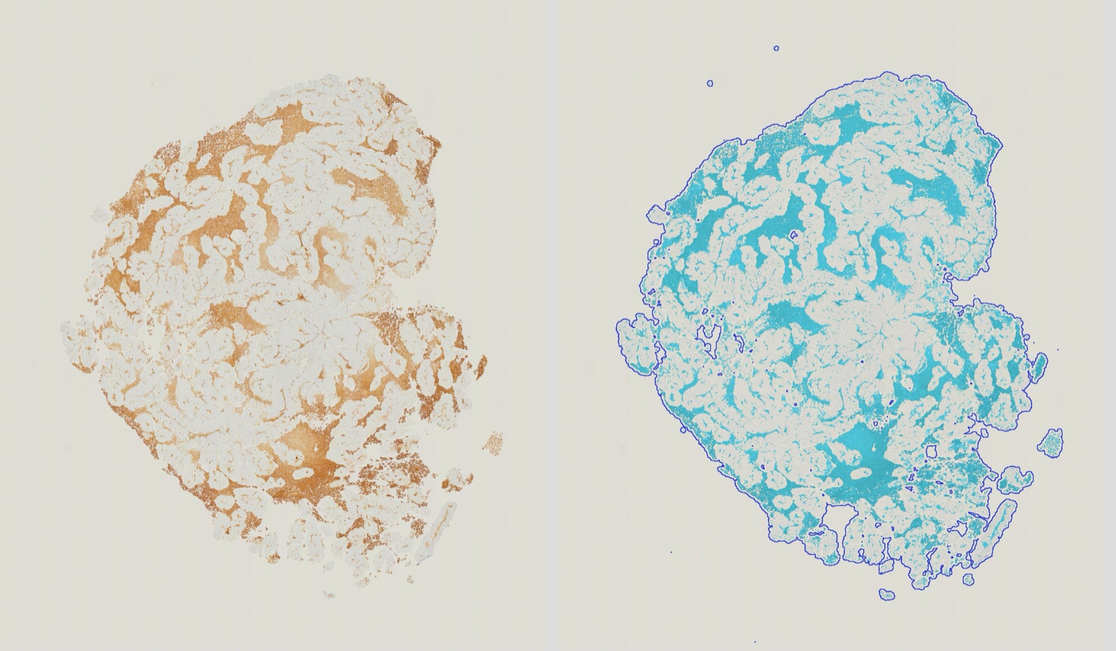
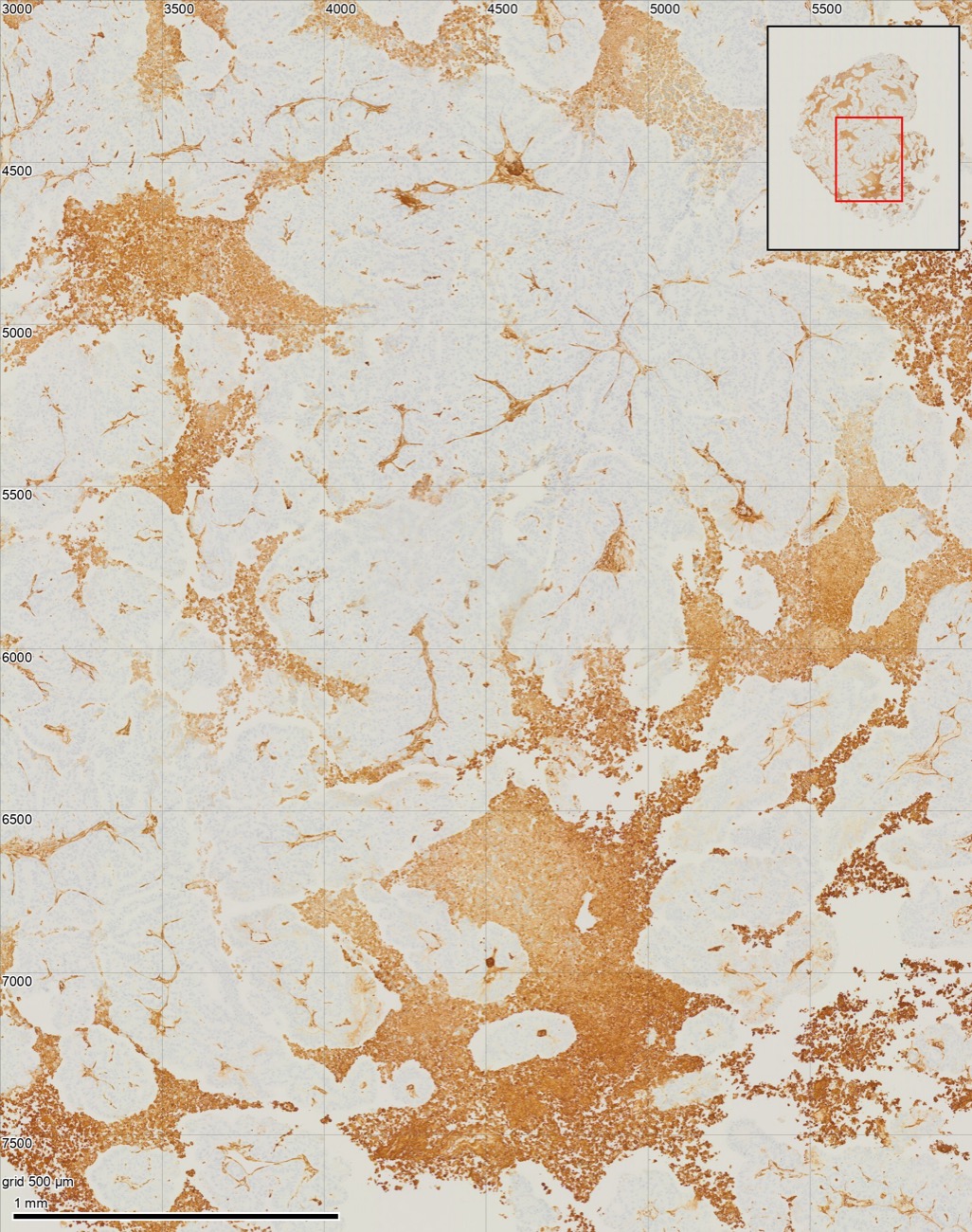
On Mouse 10 it reported 28.5% positive (9,370,272 µm² of 32,887,036 µm²). It flagged widespread brown staining in rounded, damaged-looking cells and debris as possibly non-specific (Figure 1), and noted that, as requested, this staining was counted.
3.3Measuring the study
The analysis was then fixed: the same stain separation, threshold and tissue rule for every slide, with no further choices by the model. In fixing it, the model asked whether to select non-tissue objects (the scanner's border, dust) on each slide rather than by their position on Mouse 10, and one of us said yes. The fixed analysis was run on all 57 slides. On Mouse 10 it gives 28.4%.
3.4Statistics
Agreement with the reference is reported as Pearson and Spearman correlation and as the mean difference with 95% limits of agreement [8]. Treatment groups are compared with untreated tumours by two-sided Student's t-tests (equal variances) on percent positive area. Applied to the reference values, this test gives p = 0.310, 0.097 and 0.010 for chemotherapy alone, with vardenafil and with tadalafil, against the published 0.31, 0.095 and 0.01 [6]. We also report Mann–Whitney tests.
4Results
4.1Agreement slide by slide
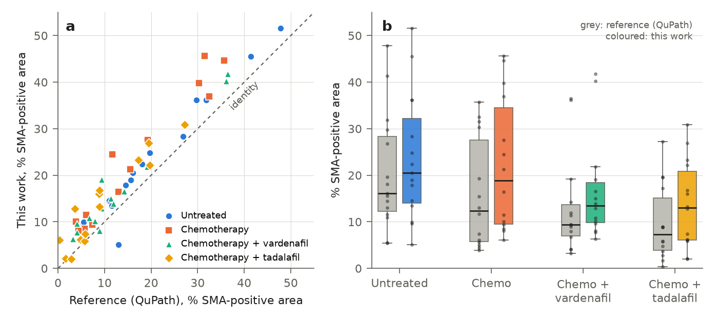
All 57 slides were measured. Percent positive area agreed closely with the reference (Figure 2a): Pearson r = 0.966, Spearman ρ = 0.918. Our values were higher by a mean of 4.3 percentage points (median 4.1), with 95% limits of agreement from −2.4 to +10.9. A linear fit gives ours = 1.07 × reference + 3.2 (R² = 0.93). For 37 of 57 slides the two values were within 5 percentage points.
The offset comes mostly from the positive area. Our positive area was a median 1.49 times the reference (Spearman ρ = 0.941). Our tissue area was a median 1.08 times the reference (Spearman ρ = 0.909). Our threshold admits fainter brown than the reference's, which thresholds a blurred image at four times coarser pixels. The two thresholds cannot be compared directly because the two analyses separate the stains differently.
4.2The study's conclusion
Table 1 and Figure 2b compare the treatment groups. Our measurements reproduce the published conclusions. Tadalafil with chemotherapy lowered α-SMA-positive area against untreated tumours (t-test p = 0.030; reference values p = 0.010). Vardenafil with chemotherapy was borderline (p = 0.146; reference p = 0.097). Chemotherapy alone made no difference (p = 0.775; reference p = 0.310). With Mann–Whitney tests, tadalafil was significant in both (p = 0.042 ours, 0.014 reference) and chemotherapy alone in neither. Vardenafil was significant in the reference (p = 0.038) and not in ours (p = 0.121).
| Median % | Mean % | |||||
|---|---|---|---|---|---|---|
| Group | n | Reference | This work | Reference | This work | p (ref. / ours) |
| Untreated | 15 | 16.1 | 20.5 | 20.5 | 23.7 | — |
| Chemotherapy | 14 | 12.3 | 18.9 | 15.8 | 22.2 | 0.310 / 0.775 |
| Chemotherapy + vardenafil | 14 | 9.4 | 13.4 | 13.1 | 16.7 | 0.097 / 0.146 |
| Chemotherapy + tadalafil | 14 | 7.3 | 13.0 | 9.6 | 13.7 | 0.010 / 0.030 |
4.3Where the two analyses differ
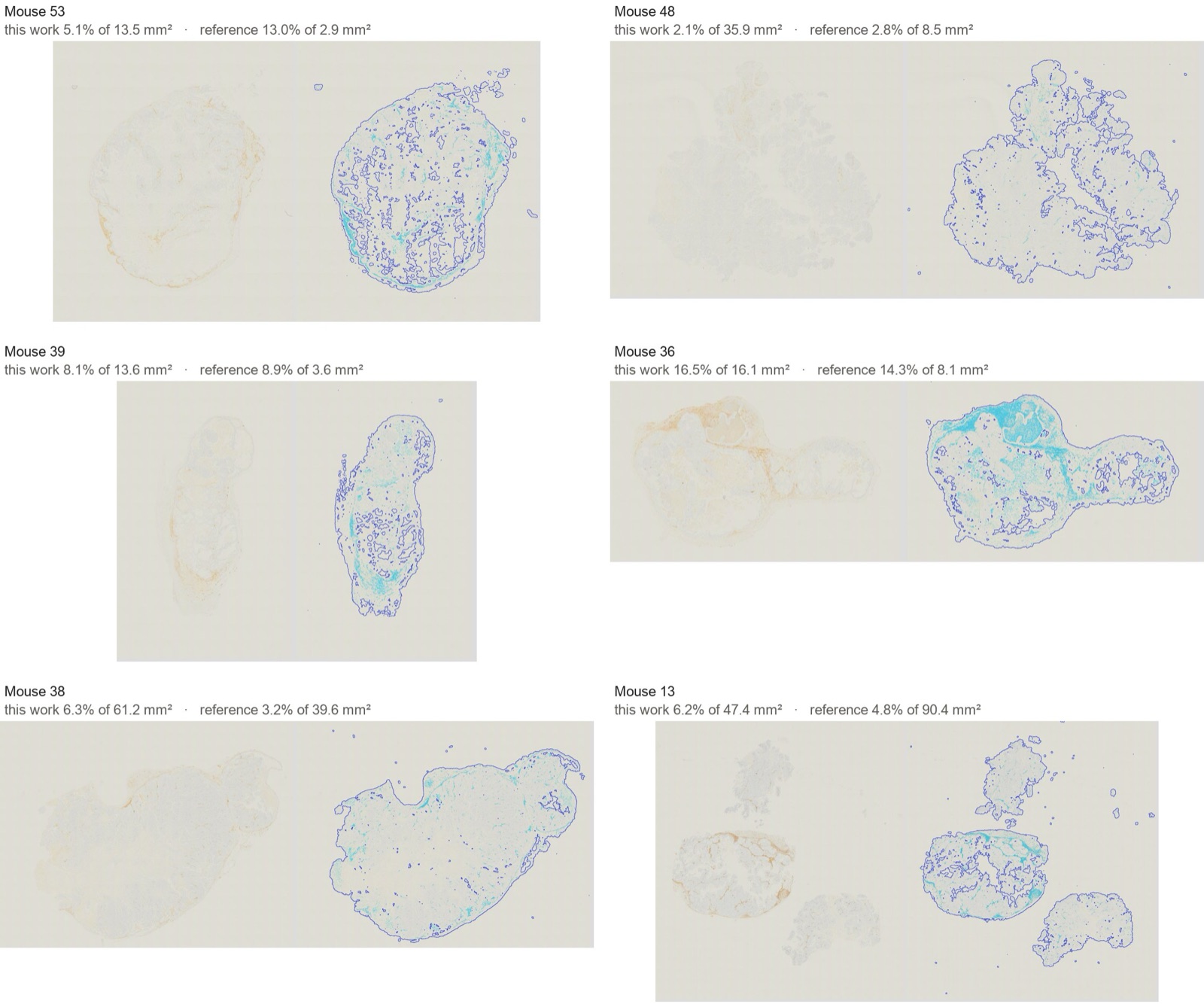
We inspected every slide where the two analyses differ most: the 11 slides whose tissue areas differ by more than a factor of 1.5, and the slides whose percent positive differs by more than 7 points. There is no ground truth for this study, so neither analysis can be called correct. The pictures do show three kinds of difference.
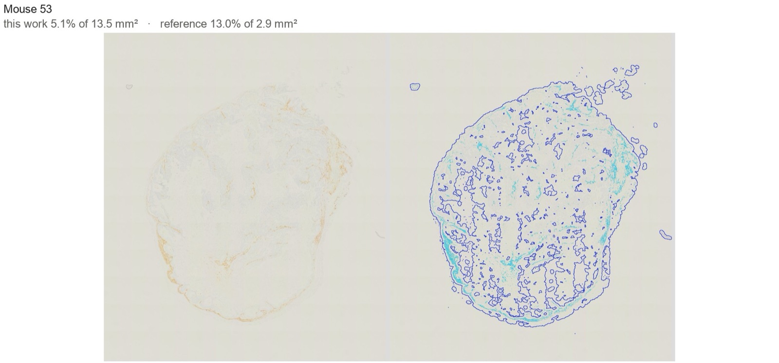
Tissue the reference left out. On 10 slides our tissue area is much larger than the reference's (Figure 3; more in Figure 4). On each of them the section is large and pale, with little counterstain, and our outline follows the whole section visible on the slide. On Mouse 53 the reference reports 2.9 mm² of tissue and we find 13.5 mm²; on Mouse 48, 8.5 mm² against 35.9 mm²; on Mouse 39, 3.6 mm² against 13.6 mm². The reference finds tissue by brightness at 20 µm per pixel, and pale tissue is close to the brightness of glass. On these slides the reference's percent positive is a share of part of the section, and we think our denominator is closer to “the whole tissue section” that both analyses set out to measure. One slide goes the other way. On Mouse 13, three separate pieces, the reference tissue area (90.4 mm²) is larger than the three pieces' outlines together (38.8 mm² with holes filled). This is consistent with the reference script growing, merging and filling the outline, which can enclose the glass between nearby pieces.
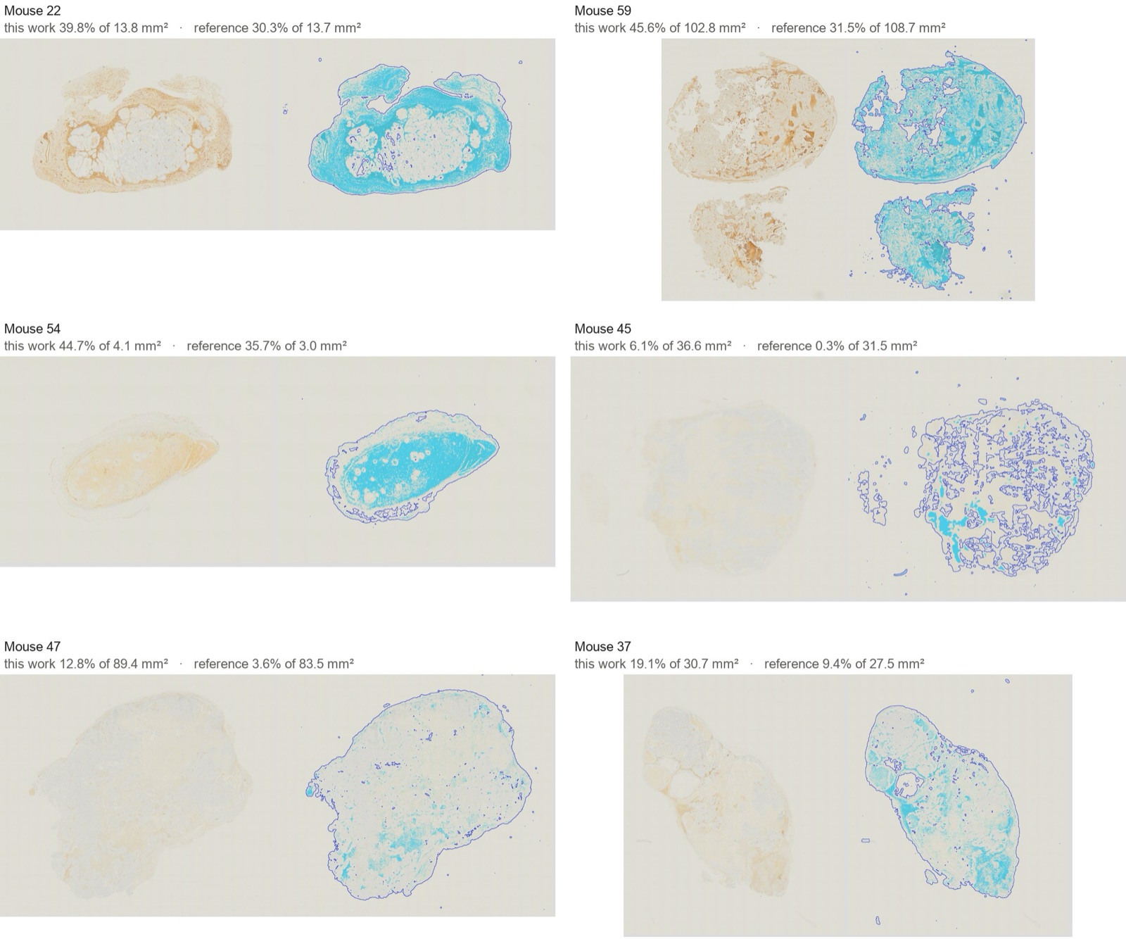
Faint brown counted by one analysis and not the other. On several slides the tissue areas agree and our positive area is larger (Figure 5, Mouse 22, 59 and 54). The extra area is visibly light brown on the slide, such as the broad band around the tumour on Mouse 22. Whether this is α-SMA or background cannot be decided from the pictures; a pathologist's reading would settle it.
Background counted as positive. Mouse 45 and Mouse 47 are weakly stained throughout, and Mouse 37 in part (Figure 5). On them our threshold counted a faint beige background as positive: 6.1% against 0.3% on Mouse 45, and 12.8% against 3.6% on Mouse 47. Here we think the reference is closer. A single threshold fixed for the study cannot tell weak specific staining from background on a slide that stained differently from the rest. A person reviewing the study would flag these slides. The study pass applied the fixed analysis without a per-slide review.
On Mouse 10, the model flagged that much of the brown staining lies in rounded, damaged-looking cells rather than in spindle-shaped fibroblasts (Figure 1b). Both analyses count this staining. If it is non-specific, both overstate fibroblast α-SMA on such slides.
4.4Time
Setup on one slide took about 3 minutes. Slides are measured independently, so the fixed analysis was run on all 57 slides in parallel, which took about 5 minutes. The whole study took about 8 minutes from request to results.
5Discussion
Given one slide and a one-sentence request, the model produced an analysis that reproduces a published study's measurements closely enough to reach the same biological conclusions. It followed the route a careful user of QuPath or Fiji would take: set the stain separation, the threshold and the tissue rule once, on slides chosen without knowing their groups, check them at full resolution, and then apply them unchanged to every slide. The threshold came from a stated rule rather than a slider, and every choice was written down where it can be checked.
The remaining differences are of two kinds. Some are choices on which reasonable analyses differ, chiefly whether pale, weakly counterstained tissue counts as tissue, and they move the denominator. Others are failures of a single fixed threshold on slides that stained differently from the rest. Both are the kind of thing a person reviewing a study checks, and a per-slide review belongs in the pipeline.
Data
The slides and reference measurements are from [7] (CC BY 4.0). Our per-slide measurements and the statistics script are released with this paper.
AFurther slides where the analyses differ
References
- P. Bankhead et al. QuPath: Open source software for digital pathology image analysis. Scientific Reports, 7:16878, 2017.
- J. Schindelin et al. Fiji: an open-source platform for biological-image analysis. Nature Methods, 9:676–682, 2012.
- A. C. Ruifrok and D. A. Johnston. Quantification of histochemical staining by color deconvolution. Analytical and Quantitative Cytology and Histology, 23:291–299, 2001.
- G. Landini, G. Martinelli, and F. Piccinini. Colour deconvolution: stain unmixing in histological imaging. Bioinformatics, 37:1485–1487, 2021.
- A. R. Crowe and W. Yue. Semi-quantitative determination of protein expression using immunohistochemistry staining and analysis: an integrated protocol. Bio-protocol, 9:e3465, 2019.
- B. P. Sharpe et al. Phosphodiesterase type 5 inhibitors enhance chemotherapy in preclinical models of esophageal adenocarcinoma by targeting cancer-associated fibroblasts. Cell Reports Medicine, 3:100541, 2022.
- A. Hayden, A. Manousopoulou, M. Cowie, R. Walker, et al. Modulation of the tumour promoting functions of cancer associated fibroblasts by phosphodiesterase type 5 inhibition increases the efficacy of chemotherapy in human preclinical models of esophageal adenocarcinoma. Zenodo, 2021. doi:10.5281/zenodo.5222122.
- J. M. Bland and D. G. Altman. Statistical methods for assessing agreement between two methods of clinical measurement. The Lancet, 327:307–310, 1986.